Algorithms

A few algorithms for Delaunay triangulation are enumerated as [Sha96] -

1.

Watson's algorithm - Watson's algorithm [Nan95] starts by forming a super-triangle which is a triangle encompassing all the given points of the domain. Initially the super-triangle is flagged as incomplete (Figures 4.2, 4.3, 4.4 and 4.5). Then the algorithm proceeds by incrementally inserting new points in the existing triangulation. A search is made for all the triangles whose circumcircles contain the new point and they are deleted to give what is known as an insertion polygon. This gives the new triangulation. This process is continued till all points to be inserted are exhausted and then all triangles having the vertices of the super-triangle are deleted.

  

Figure 4.2: Watson's algorithm : Initial triangulation

  

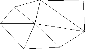Figure 4.3: Watson's algorithm : Point insertion

  

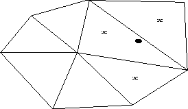Figure 4.4: Watson's algorithm : Element deletion

  

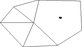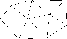
Figure 4.5: Watson's algorithm : Final mesh

This is one of the simplest and the most extensively used algorithm for Delaunay triangulation.

2.

Lawson's algorithm or the diagonal swapping algorithm - If a point is added to an existing triangular mesh then circumcircles are formed for all new triangles formed. If any of the neighbours lie inside the circumcircle of any triangle, then a quadrilateral is formed using the triangle and its neighbour. The diagonals of this quadrilateral are swapped to give a new triangulation. This process is continued till there are no more faulty triangles and no more swaps are required.

3.

Fang and Piegl algorithm - This algorithm for triangulation places the given points in a uniform mesh and creates triangles in a circular manner. The authors claim a linear time complexity for the algorithm. The algorithm also produces the convex hull of the given set of points at no extra cost. The algorithm is so designed that points only on one side the current point under consideration have to be checked for the Delaunay criterion. However, this algorithm runs into troubles when too many points lie on a straight line.

4.

Constrained Delaunay Triangulation (CDT) - If a set of points in a plane and a set of non-crossing edges are specified then the CDT creates a mesh such that -

(a)

All the specified edges are included in the triangulation.

(b)

It is as close to Delaunay triangulation as possible.

This algorithm has been tested to work in a time complexity of $O(N \log N)$for N specified points in the domain. If a set of points and non-crossing edges are specified then the CDT of the given set has the property that for all new edges there exists a circle such that,

• the endpoints of the edge lie on the circle, and
• if any new node is in the circle, then it is invisible from at least one of the nodes of the edge, i.e., if lines are drawn from the point to the two nodes of the edge then at least one of them will intersect with one of the edges of the mesh.

Thus, if no edges are specified, the CDT is the same as Delaunay triangulation. CDT is a divide-and-conquer algorithm since the given data is sorted according to any one dimension and the domain is divided into strips. The CDT for each strip is then calculated and pasted to form new strips whose CDT is then calculated. This process is repeated till the CDT for the entire domain is obtained.

5.

Sweepline algorithm - In a Voronoi tessellation, a sweepline is defined as the intersection of a moving horizontal line with the Voronoi boundaries. Circumcircles are located by finding the point of intersection of three bisectors of the lines joining the nodes. But the Voronoi polygons obtained this way are not very robust and there have been only a few attempts to tackle this problem. A one-to-one geometric transformation maps a bisector onto a hyperbola or a vertical half-line. Any bisector between any two nodes, say p and q, is mapped as

The transformation maps x as such and y as the original value and the distance between the point and the node p. The mapped Voronoi regions R_p^* and R_q^* are bounded by the mapped bisector, say C_pq, which is either a hyperbola or a straight half-line. A bisector is generated only if the sweepline has reached both forming nodes. An expected vertex is the intersection point of two neighbouring bisectors.